Neural Networks from Scratch — part 2 Chaining Neurons

Welcome again! This is a continuation of the previous guide. If you haven’t seen it, please go through it once. In this guide, we’ll be doing a lot of work. Our main goal is to chain neurons together, meaning the output of one neuron becomes the input of the next. Right now, we will still have a linear chain of neurons (no layers), so the network is still pretty basic. But this lays the important groundwork for the future.
Trying to model a squared relationship
We’ll be using the neuron created in the previous guide. It could successfully track linear relationships between two variables. But, what if we change that relationship?
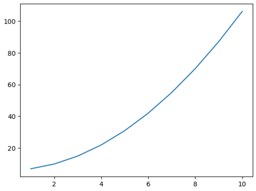
Suppose we have two variables: xand y, where ydepends on the square of x:
x = np.array([i for i in range(1, 11)])
y = x**2 + 6
Its graph looks like this:
If we train the same neuron on this data and plot its output, we get the following:
pred = [n1.forward(i)[0] for i in x]
plt.plot(x, y)
plt.plot(x, pred)
plt.show()
It tried its best but failed. The model can only map linear relationships. If we want it to map other nonlinear relationships, we need to do something.
Chaining neurons together
Maybe it’s because there’s only one neuron. If we add more neurons, we might be able to get some complexity. Let’s try to implement that.
If we add one more neuron, our network will look like this:

It has two hidden neurons. The equations should just repeat themselves:

Notice now we have 4 parameters: the weight and bias for the first neuron and the weight and bias for the second neuron. Also, notice that the output of the first neuron z1becomes the input of the next neuron.
Updating the Backward Function
Our gradient calculation now has twice as many equations. But that’s no big deal since they’re just the same equations repeated twice. We’ll update the backward function in our Neuron class to work for both neurons.
For reference, this was the previous function:
    def backward(self, pred, y, learning_rate):
        # Getting the derivatives
        dLdz = mse_deriv(pred, y)
        dzdw = self.x
        dzdb = 1

        # These are the first and second terms of the gradient vector
        dLdw = -dLdz * dzdw
        dLdb = -dLdz * dzdb

        # Updating our weight and bias
        self.w += learning_rate * dLdw
        self.b += learning_rate * dLdb
Here’s how we’ll do it:
- Change Parameters: Take in an error instead of prediction and actual values.
- Update Weights and Biases: Use gradient descent.
- Propagate Error: Find the error to be sent to the previous layer.
    def backward(self, error, learning_rate):
        # Getting the derivatives
        dzdw = self.input
        dzdb = 1

        # These are the first and second terms of the gradient vector
        dLdw = -error * dzdw
        dLdb = -error * dzdb

        # Updating our weight and bias
        self.w += learning_rate * dLdw
        self.b += learning_rate * dLdb

        # The error of the previous layer
        return self.w
The code is almost the same. I’ve taken the dLdz = mse_deriv(pred, y) line out. This will be inputted as the error parameter. The only other thing I added was return self.w
Explanation of Error Propagation
If you’re confused how this happened, look at the following reasoning:
The partial of the cost with respect to the weight and bias of the second neuron is already calculated. We need to find the partial of the cost with respect to the previous neuron’s parameters.
To calculate the loss, we need to calculate z2. To calculate z2, we need z1, and to calculate z1, we need w1. So the chain rule comes out to be:

But, z1 and z2 are linearly related (Look at the formulae again). So,

This is why we return self.w. This value is returned so that we can send it to the first neuron.
Training the Network
Here’s what the training code looks like now:
n1 = Neuron()
n2 = Neuron()
learning_rate = 0.0001
epochs = 10000

for epoch in range(epochs):
    total_error = 0  # This is to calculate the average error over all the data

    # Running the training
    for i in range(len(x)):
        # Forward
        z1 = n1.forward(x[i])
        z2 = n2.forward(z1)

        # Error
        total_error += mse(z2, y[i])

        # Backward
        dLdz2 = mse_deriv(z2, y[i])
        dLdz1 *= n2.backward(dLdz2, learning_rate)
        n1.backward(change, learning_rate)

    # Getting the average error
    if epoch % 50 == 0:
        print(f"epoch = {epoch}, error = {round(total_error / len(x), 3)}")
The only change is in the Backwards part. As I’ve said, I’ve taken out the mse_deriv part outside the function. Then I run the n2.backward() function and multiply it with the error and then send it to n1.backward() . Why did this happen?
n2.backward() returns the partial of z2 with respect to z
But, the entire formula was:
So we need to multiply that term by the partial of L with respect to z2 and the partial of z1 with respect to w1. And, our error variable is precisely the first term. So, we multiply them together to get the partial of L with respect to z1. Finally, the last term will be multiplied in the first neuron, so that’s already taken care of. You can run the train function to see that the network is indeed learning. This means we got the math right.
Refactoring the code to work with any number of neurons
Now that all the math is done, we can refactor the code to work with any number of neurons. First of all, let’s create an MSE class to keep the MSE function and its derivative packaged together. This will replace the mse and mse_deriv functions we created before
class MSE:
    def forward(self, a, y): return np.power(a - y, 2).mean()

    def backward(self, a, y): return 2 * (a - y)
Next, let’s create a new class called “Network”. We will take in a list of neurons and the loss function (in this case, it is MSE)
class Network:
    def __init__(self, neurons, activations, loss_function):
        self.neurons = neurons
        self.loss_function = loss_function
Then we can add a forward function, that iteratively runs the forward command of each neuron and sends the output to the next:
class Network:
    ...
    def forward(self, x):
        for n in self.neurons:
          x = n.forward(x)
        return x
    ...
Then we add a backward function for the back-propagation part:
class Network:
    ...
    def backward(self, error, learning_rate):
        for i in range(len(self.neurons), 0, -1):
            error = self.neurons[i - 1].backward(error, learning_rate)
    ....
Finally, we can add a train function:
def train(self, training_data, training_labels, learning_rate, epochs):
    for epoch in range(epochs):
        total_error = 0

        # Running the training
        for i in range(len(training_data)):

            a = self.forward(training_data[i])

            total_error += self.loss_function.forward(a, training_labels[i])

            self.backward(self.loss_function.backward(a, training_labels[i]), learning_rate)

        if epoch % (epochs / 10) == 0:
            print(
                f"epoch = {epoch}, error = {round(total_error / len(training_data), 3)}"
            )
In the training loop, we run the forward function to get our predicted value, use the loss function to calculate our error, and then use the backward function to update the network.
Entire Network class:
class Network:
    def __init__(self, neurons, loss_function):
        self.neurons = neurons
        self.loss_function = loss_function

    def forward(self, x):
        for n in self.neurons:
            x = n.forward(x)
        return x

    def backward(self, error, learning_rate):
        for i in range(len(self.neurons), 0, -1):
            error = self.neurons[i - 1].backward(error, learning_rate)

    def train(self, training_data, training_labels, learning_rate, epochs):
        for epoch in range(epochs):
            total_error = 0

            # Running the training
            for i in range(len(training_data)):
                a = self.forward(training_data[i])
                total_error += self.loss_function.forward(a, training_labels[i])
                self.backward(
                    self.loss_function.backward(a, training_labels[i]), learning_rate
                )

            if epoch % (epochs / 10) == 0:
                print(
                    f"epoch = {epoch}, error = {round(total_error / len(training_data), 3)}"
                )
We can test out the network:
network = Network([Neuron()], MSE())

network.train(x, y, learning_rate=0.001, epochs=100)
In this case, we create a network with 1 neuron and use the MSE loss function, then we run the train function.
epoch = 0, error = 1702.332
epoch = 10, error = 122.188
epoch = 20, error = 116.771
epoch = 30, error = 111.767
epoch = 40, error = 107.177
epoch = 50, error = 102.969
epoch = 60, error = 99.109
epoch = 70, error = 95.571
epoch = 80, error = 92.327
epoch = 90, error = 89.352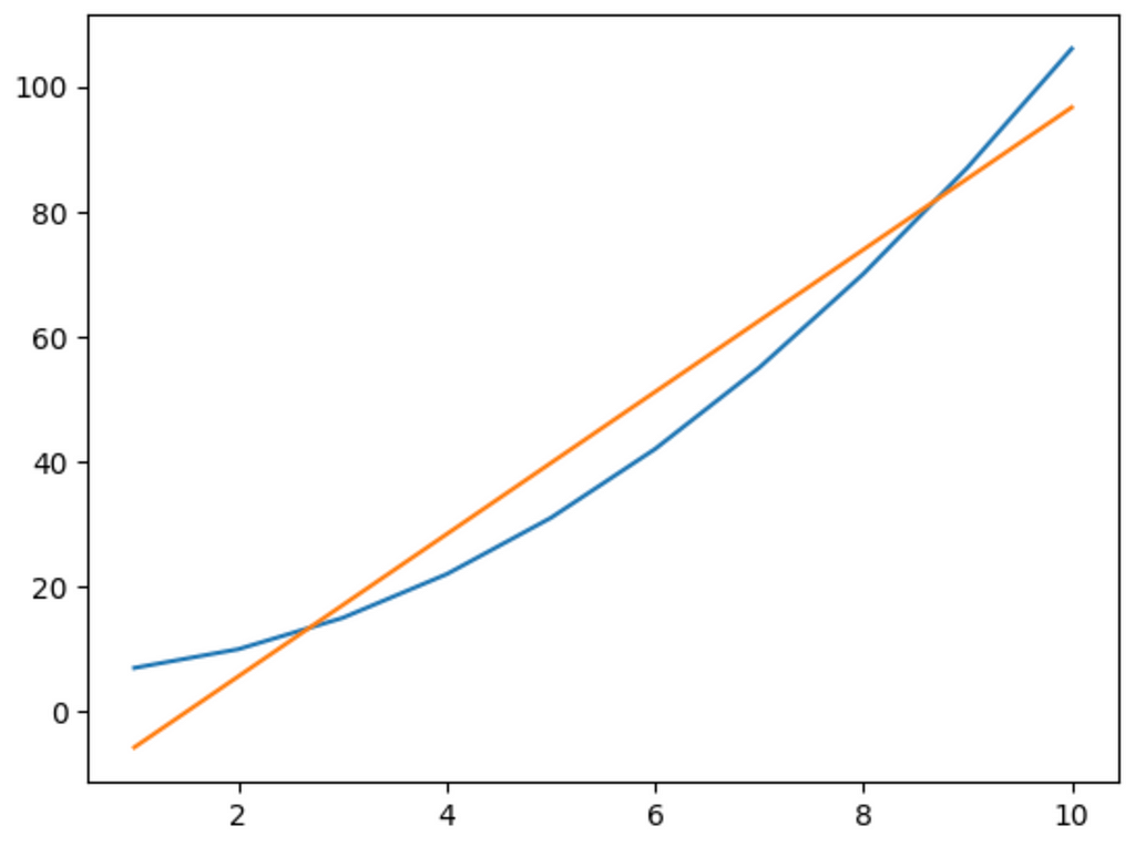
Conclusion
Unfortunately, we have the same problem. You can test the code by adding 5 or 10 neurons in a chain, and the network will always produce a linear output. This shows that just adding more neurons doesn’t necessarily add complexity; we need to add something else. In the next guide, we’ll look into activation functions to fix this problem. Stay tuned!